Phillips Curve, Historical Background, Framework, Examples

The Phillips Curve is a foundational concept in economics that examines the relationship between inflation and unemployment. It explains that there is an inverse relationship between the two variables: when unemployment is low, inflation tends to rise, and conversely, when unemployment is high, inflation remains subdued. This theory has influenced economic policymaking around the world, helping governments and central banks balance employment generation with price stability. In this article, we are going to cover the Phillips Curve, its historical background, theoretical framework, examples, importance and limitations. 

Phillips Curve

The Phillips Curve connects two most important components of any economy: inflation and unemployment. Inflation refers to the rate at which prices of goods and services increase over time, reflecting the rising cost of living. Unemployment measures the number of people who are willing and able to work but cannot find employment. According to the Phillips Curve, low unemployment leads to higher inflation because more people earning wages increases consumer spending, which drives up demand and, consequently, prices. Conversely, high unemployment reduces overall spending, keeping demand and prices lower.

This relationship makes the Phillips Curve a valuable tool for policymakers, allowing them to understand the trade-offs involved in pursuing full employment while maintaining price stability. It serves as a guide for monetary and fiscal measures that influence both employment and inflation.

Phillips Curve Historical Background

The concept of the Phillips Curve was introduced by A.W. Phillips, a New Zealand-born economist, who in 1958 published a paper titled “The Relationship Between Unemployment and the Rate of Change of Money Wage Rates in the United Kingdom, 1861-1957.” Phillips analyzed nearly a century of data from the UK and discovered a clear inverse relationship between wage inflation and unemployment. He observed that when unemployment was low, wages rose rapidly, whereas high unemployment led to slower wage growth.

In the starting, the analysis focused on wage inflation. However, economists soon extended Phillips’ work to general price inflation, applying the concept to broader economic policy. During the 1960s, the Phillips Curve gained acceptance everywhere, specially in the United States, where policymakers used it as a tool to manage economic growth and inflation. The theory, however, faced challenges during the 1970s when many countries experienced stagflation that was a combination of high inflation and high unemployment which contradicted the original premise of the Phillip’s curve.

‹ ›

Phillips Curve Theoretical Framework

The Phillips Curve theory is based on a trade-off between inflation and unemployment:

• Low unemployment = High inflation: With more people employed, aggregate spending rises, driving up demand and increasing prices.
• High unemployment = Low inflation: Fewer people earning wages reduces spending, lowering demand and keeping prices stable.

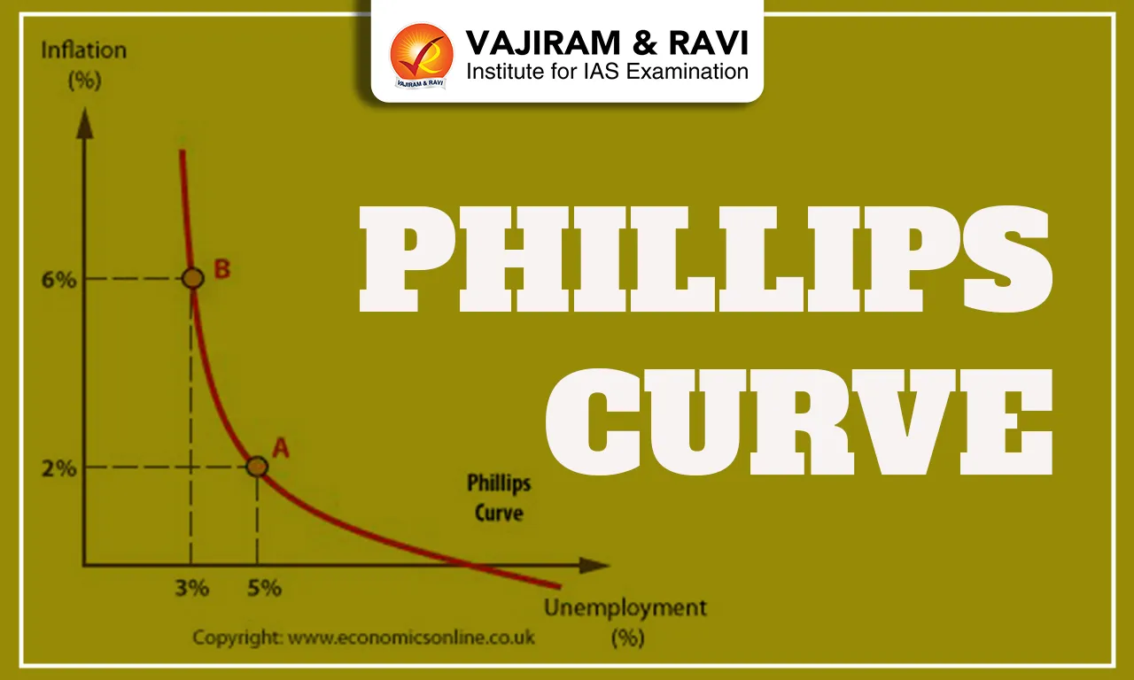
Graphically, the Phillips Curve is represented as a downward-sloping curve, illustrating the inverse relationship between the two variables. Policymakers once believed they could select a point on this curve depending on their priorities: reducing unemployment would mean accepting higher inflation, while controlling inflation would require tolerating higher unemployment. 

Over time, economists refined the theory to account for expectations. The expectations-augmented Phillips Curve suggests that anticipated inflation influences wage-setting and price behavior, weakening the apparent trade-off in the long run. Similarly, the long-run Phillips Curve indicates that the economy naturally returns to its “natural rate of unemployment,” irrespective of inflation, meaning the original inverse relationship is not sustainable over extended periods.

Phillips Curve Examples 

1. United States in the 1960s: The U.S. economy in the beginning seemed to validate the Phillips Curve. Low unemployment coincided with rising inflation, and policymakers believed they could reduce unemployment further by tolerating moderate inflation.
2. United States in the 1970s (Stagflation): This period challenged the Phillips Curve. The U.S. faced both high inflation and high unemployment at the same time demonstrating that the trade-off does not always hold. Stagflation highlighted the need to incorporate supply-side shocks and expectations into the analysis.

Phillips Curve Limitations

While the Phillips Curve remains an important analytical tool, it has many limitations. These limitations include: 

• Ignores expectations: Individuals and businesses adjust their behavior if they anticipate inflation, diminishing the effectiveness of the trade-off.
• Fails in the long run: Over time, unemployment tends toward its natural rate, making inflation ineffective in reducing unemployment.
• Cannot explain stagflation: The simultaneous rise of inflation and unemployment in the 1970s exposed the curve’s shortcomings.
• Vulnerability to supply-side shocks: External factors such as oil crises, wars, or pandemics can disrupt both inflation and unemployment independently.
• Context-specific assumptions: The curve may not apply universally across different economies or economic conditions.

These limitations indicate that while the Phillips Curve is valuable for understanding short-term trends, it must be used alongside other analytical tools for comprehensive policy formulation.

Phillips Curve Importance and Policy Implications

Despite its limitations, the Phillips Curve continues to hold relevance in economics and policymaking:

• Framing policy decisions: Central banks, including the Reserve Bank of India and the U.S. Federal Reserve, use the Phillips Curve to avoid the effects of interest rate adjustments on employment and inflation.
• Understanding short-term dynamics: In the short run, the curve may provide useful insights into the relationship between wage pressures and price changes.
• Encouraging balanced policymaking: Policymakers are reminded of the trade-offs between controlling inflation and promoting employment, fostering better decision-making.

Influencing wage negotiations: Both employers and employees may use Phillips Curve insights to inform salary adjustments based on expected inflation and labor market conditions.